Developed a tire model to simulate longitudinal dynamics of a vehicle. This was part of the Vehicle Dynamics class I took at university.
First a model for slip was created using the Pacejka model.
μ(k)=c1⋅(1−e−c2⋅k)−c3⋅k
Where k is the braking slip ratio, c1 is the asymptote of the curve, c2 is the shape factor, and c3 is the curvature factor.
The Pacejka model was then used to create a model for the longitudinal force of the tire.
Using newton's second law, on the vehicle body:
m⋅x¨FL∴FB=−FB−FL=cw⋅A⋅2ρ⋅x˙2=−m⋅x¨−cw⋅A⋅2ρ⋅x˙2
Wheremx¨FBFLcwAρx˙:mass of the vehicle:acceleration of the vehicle:braking force:drag force:drag coefficient:frontal area of the vehicle:density of air:velocity of the vehicle
Similarly using newton's second law on the wheel:
JW⋅θ¨wFBFNk=FB⋅rw−MB=μ(k)⋅FN=m⋅g=x˙x˙−rw⋅θ˙w
WhereJWθ¨wMBrwFNg:moment of inertia of the wheel:angular acceleration of the wheel:braking torque:radius of the wheel:normal force:acceleration due to gravity
These relationships can be modeled in Simulink as shown below:
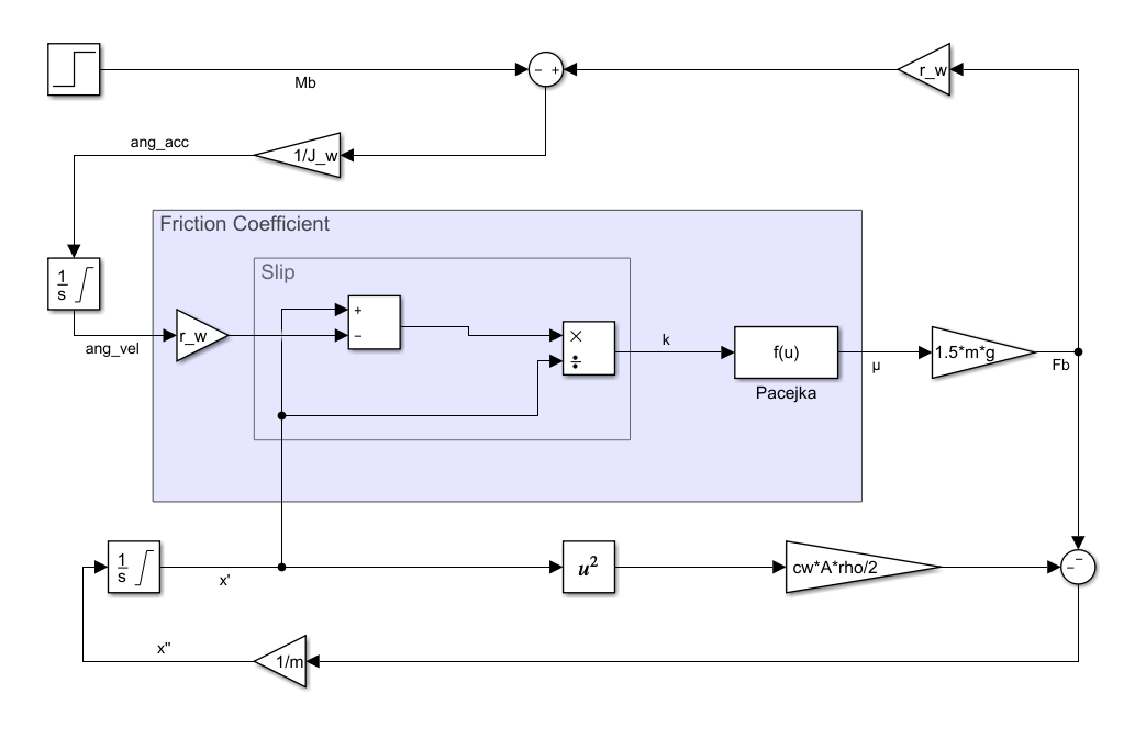
This model was used as a basis for the ABS system. The system simply compares the slip with an ideal slip parameter and changes the applied dynamic braking torque.
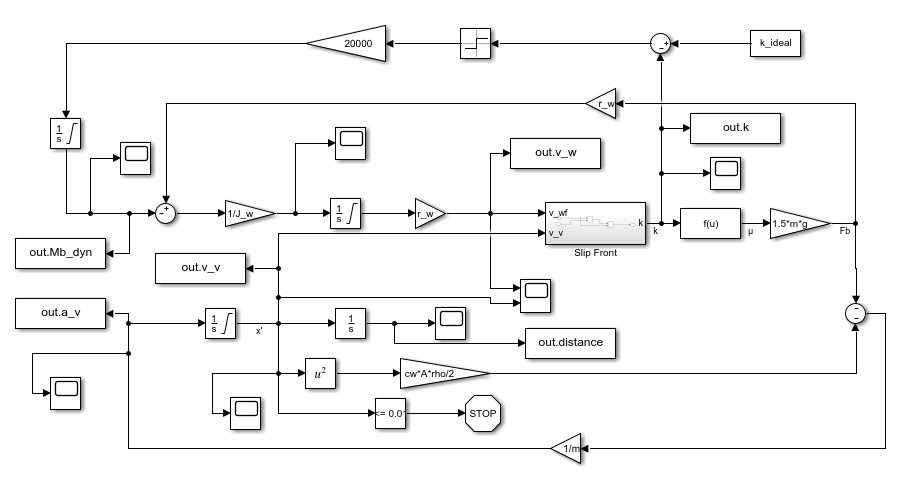
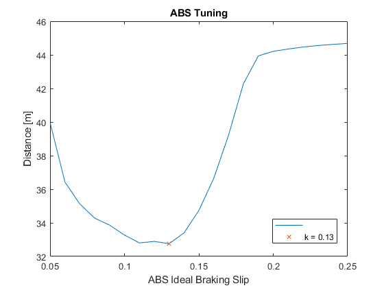
This model was used to find an ideal slip parameter for the vehicle. The ideal slip parameter was found to be 0.13.
close all
clear all
param;
k = 0.05:0.01:0.25;
for i = 1:21
k_ideal = k(i);
out = sim('brakingabs.slx');
D(i)=out.distance(end);
end
[MIN,IND]=min(D);
figure(1)
plot(k,D)
hold on
xlabel('ABS Ideal Braking Slip')
ylabel('Distance [m]')
title('ABS Tuning')
plot(k(IND),D(IND),'x')
legend('','k = 0.13')
hold off
abs = sim('brakingabs.slx');
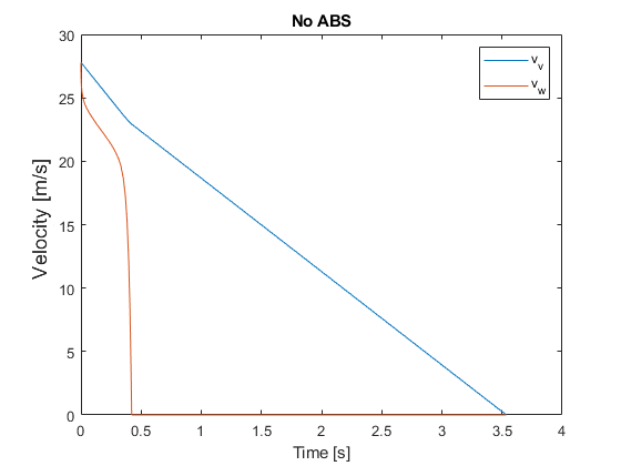
noabs = sim('braking.slx');
The following graphs show the performance of the ABS function.